i-Tree Cool Air Model Methods

1. Overview

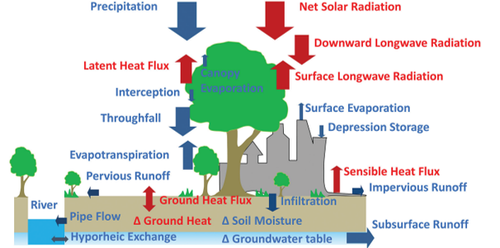
i-Tree Cool Air simulates near-surface air temperature, humidity, and heat-stress conditions across urban landscapes. For every grid cell and time step, the model solves a coupled radiation-energy-moisture balance, resolving how each land-cover component (tree canopy, short vegetation, impervious surfaces, bare soil, and open water) exchanges heat and water with the overlying atmosphere. These per-cover fluxes are area-weighted within each pixel and linked to a mesoscale atmospheric boundary, producing spatially continuous fields of air temperature, humidity, and human heat-stress indicators across the modeling domain.

The model traces its intellectual core to Yang et al. (2013), who developed a physically based analytical framework for spatial air temperature and humidity in urban landscapes. That framework has since been substantially extended within the HydroPlus research suite to include the urban water balance, snow hydrology, green infrastructure representation, street-canyon radiation geometry, seasonal phenological dynamics, and human thermal comfort metrics.

Results are produced at the native grid resolution (for example, 30 m) and can be aggregated to reporting units such as U.S. Census block groups, supporting analysis at both neighborhood and city scale.

1.1 Model Architecture: Physics-Based and Parameterized Components

At its core, the model is built around a three-layer system linking a mesoscale atmospheric boundary to the urban canopy air layer and the land surface, drawing on a range of established and original methods to represent heat, water, and momentum exchange at each grid cell and time step.

Physics-Based Components

The following processes are resolved from governing equations of mass, energy, and momentum exchange:

• Surface Energy Balance (SEB). The model partitions net all-wave radiation (Rn) into sensible heat (H), latent heat (LE), urban heat storage flux (△Qs), and anthropogenic heat emission (QF), expressed as Rn = H + LE + △Qs + QF (Yang et al., 2013). Fluxes are computed separately for trees, short vegetation, impervious surfaces, bare soil, and open water, then combined by fractional area within each grid cell.
• Urban Canyon Radiation. Shortwave radiation absorbed by road, wall, garden, and roof surfaces is resolved through a multi-reflection scheme accounting for direct and diffuse components, sky-view factors, and canyon aspect ratio (building height to street width), following and extending the Town Energy Balance framework (Masson, 2000). Longwave exchange is computed per surface using emissivity and estimated surface temperature via Kirchhoff's law.
• Aerodynamic Resistance Networks. Turbulent exchange of heat and moisture between each surface type and the atmosphere is governed by aerodynamic resistance (ra, s m^-1) derived from wind speed, roughness length, zero-plane displacement, and atmospheric stability (Choudhury and Monteith, 1988; Yang and Endreny, 2013). Stomatal resistance (rs) for trees and short vegetation is parameterized as a function of LAI, BAI, and vapor pressure deficit.
• Soil-Vegetation-Atmosphere Transfer (SVAT). Evapotranspiration from trees and short vegetation is computed using the Penman-Monteith equation, with separate treatment of canopy evaporation (from intercepted water, governed by ra only) and transpiration (governed by both ra and rs) (Allen et al., 1998). Infiltration is computed using the Green-Ampt method.
• Canopy Interception and Snow Hydrology. Rainfall interception and throughfall are computed using the sparse Rutter model, with canopy storage capacity based on LAI, BAI, and per-unit storage depths for leaves and bark (Valente et al., 1997). Snow accumulation, melt, and sublimation are resolved separately for open-area ground, under-tree, and under-short-vegetation conditions.
• Analytical Spatial Air Temperature and Humidity Model. Following Yang and Endreny (2013), the model couples the urban canopy air layer to a mesoscale atmospheric boundary through a system of governing equations, iteratively solving for local-cell air temperature and absolute humidity from the combined surface energy and moisture fluxes.

Parameterized Components

The following components use empirically calibrated relationships in place of full process equations:

• Ground Heat Storage (Objective Hysteresis Model). Urban storage heat flux (△Qs) is estimated using the Objective Hysteresis Model (Grimmond and Oke, 1999; Sun et al., 2017), which relates storage flux to net radiation through empirically derived coefficients.
• Radiative Surface Properties. Longwave emission and albedo are parameterized by land-cover type using observed datasets for urban materials, with albedo adjusted for solar zenith angle.
• Anthropogenic Heat Emissions. Heat from buildings, traffic, and human metabolism (QF, W m^-2) is represented using diurnal and monthly scaling factors fitted to observed rates.
• Seasonal Vegetation Phenology. LAI and BAI for tree and short-vegetation cover vary through the year following empirically fitted leaf-on and leaf-off transition curves.

2. Model Applications

Cool Air is designed not only to simulate existing urban temperature patterns, but also to simulate temperature changes with land-use characteristics. By resolving energy and water exchanges from first principles at every grid cell, the model quantifies how individual land-cover components contribute to heat generation and dissipation.

3. Model Steps

Cool Air advances through time in hourly or sub-hourly steps. At each time step, the simulation loops through every grid cell in the domain in spatial order, executing the full sequence of calculations.

Before the time loop begins, the model initializes LAI/BAI phenology schedules and pre-processes weighted meteorological inputs when multiple weather stations are provided.

Step 1: Meteorological Forcing Initialization

Meteorological inputs (air temperature, dew-point temperature, pressure, shortwave/longwave radiation, wind speed, and precipitation) are read as time-series data from one or more stations. When multiple stations are provided, inputs are spatially interpolated and lapse-rate adjusted.

Step 2: Mesoscale Atmospheric Boundary Initialization

Observations at the reference station establish mesoscale background air temperature and absolute humidity for the shared atmospheric layer above the urban canopy.

Step 3: Pixel-Level Energy Balance

For each grid cell, the model computes surface energy balance across all land-cover components. Net radiation is calculated for trees, short vegetation, impervious surfaces, bare soil, and open water.

Rn = H + LE + △Qs + QF

Net radiation (Rn, W m^-2) is partitioned into sensible heat (H), latent heat (LE), urban heat storage (△Qs), and anthropogenic heat (QF).

Step 4: Hydrologic and Vegetation Processes

Water balance components are updated in the following sequence for each grid cell:

• Potential evapotranspiration is computed using Penman-Monteith.
• Canopy interception and throughfall are computed with the sparse Rutter model.
• Canopy evaporation is computed for intercepted water.
• Snow ablation is computed for open-area, under-tree, and under-short-vegetation conditions.
• Surface inflows are routed to impervious/pervious depression and open water storage.
• Infiltration is computed using Green-Ampt.
• Lateral groundwater redistribution is resolved across topographic-index bins.
• Root-zone ET, drainage, saturation-excess runoff, and subsurface runoff are computed in sequence.
• If GI devices are present, inflow/infiltration/drainage/overflow are computed separately.

Step 5: Atmospheric State Update

Near-surface air temperature and absolute humidity are solved from combined surface energy fluxes and resistance networks. For non-reference pixels, a Levenberg-Marquardt iterative method solves local canopy-layer conditions consistent with boundary conditions.

Step 6: Heat Metrics, Routing, and Output

Heat-stress indicators (Heat Index, Humidex, WBGT, UTCI, and Wind Chill) are computed from modeled conditions at each pixel. Surface runoff is routed across the domain and outputs are written as spatial maps and time series.

4. Model Inputs and Outputs

4.1 Required Inputs

Meteorological Forcing. Time-varying weather data including temperature, humidity/dew point, pressure, shortwave and longwave radiation, wind speed, and precipitation.

Land Surface and Urban Characteristics. Spatial rasters describing tree cover, short vegetation, impervious fractions, bare soil, and open water, along with urban geometry parameters.

Vegetation Parameters. LAI, BAI, storage capacities, phenology schedules, and related canopy parameters.

Soil and Hydrologic Parameters. Conductivity, moisture thresholds, infiltration parameters, and topographic index distributions.

Surface Radiative Properties. Albedo and emissivity values by land-cover type, plus Objective Hysteresis coefficients.

Anthropogenic Heat and Additional Inputs. Anthropogenic heat estimates with diurnal/monthly scaling, a DEM for lapse-rate/routing, and GI parameters when used.

4.2 Model Outputs

The model generates spatially distributed outputs at each grid cell and time step. Map outputs are written in ArcGIS ASCII raster format and time series are written as CSV files.

Atmospheric State

• Near-surface air temperature (Tair) and dew-point temperature (Tdew)
• Absolute humidity
• Mesoscale background temperature and humidity

Energy Fluxes (Pixel Totals)

• Net radiation, sensible heat, latent heat, urban heat storage flux, and anthropogenic heat

Energy Fluxes (Per Land-Cover Component)

• NR, H, LE, and △Qs for impervious, tree, short vegetation, soil, and water cover
• Tree and short-vegetation latent heat split into evaporation and transpiration

Water Balance

• Canopy interception storage and evaporation
• Snow water equivalent, melt, and sublimation outputs
• Depression storage on impervious, pervious, and water surfaces
• Infiltration, storage deficits, ET, and subsurface runoff
• Surface runoff and routed streamflow
• GI inflow, infiltration, drainage, and overflow (when active)

Human Heat-Stress Metrics

• Heat Index
• Humidex
• Wet Bulb Globe Temperature (WBGT)
• Natural wet-bulb and psychrometric wet-bulb temperature
• Globe temperature
• Universal Thermal Climate Index (UTCI)
• Wind Chill

Aerodynamic and Resistance Diagnostics

• Aerodynamic resistance for tree, short vegetation, impervious, soil, and water cover
• Wind speed at canopy level

Aggregated Outputs

• All variables aggregated to U.S. Census block groups (daily and hourly)
• Catchment-total water balance and energy flux summaries
• Water-quality loading and removal summaries when pollutant tracking is enabled

References

• Allen, R.G., Pereira, L.S., Raes, D., et al. (1998). Crop evapotranspiration: FAO Irrigation and Drainage Paper 56.
• Choudhury, B.J. and Monteith, J. (1988). A four-layer model for the heat budget of homogeneous land surfaces.
• Grimmond, C. and Oke, T.R. (1999). Heat storage in urban areas: observations and simple model evaluation.
• Hirabayashi, S. and Nowak, D.J. (2016). National database of tree effects on air quality and health.
• Liljegren, J.C., Carhart, R.A., Lawday, P., et al. (2008). Modeling wet bulb globe temperature.
• Masson, V. (2000). A physically based scheme for the urban energy budget in atmospheric models.
• Oke, T., Mills, G., Christen, A., et al. (2017). Urban Climates.
• Rothfusz, L. (1990). The heat index equation (NWS technical attachment SR 90-23).
• Steadman, R.G. (1979). The assessment of sultriness, Part I.
• Stull, R.B. and Ahrens, C.D. (2000). Meteorology for scientists and engineers.
• Sun, T., Wang, Z.-H., Oechel, W.C., et al. (2017). AnOHM v1.0 bulk storage heat flux coefficients.
• Valente, F., David, J. and Gash, J. (1997). Interception loss modeling for sparse forests.
• Wang, J., Endreny, T.A. and Nowak, D.J. (2008). Mechanistic simulation of tree effects in an urban water balance model.
• Ward, H.C., Kotthaus, S., Jarvi, L., et al. (2016). Surface Urban Energy and Water Balance Scheme (SUEWS).
• Yang, F., Mitchell, K., Hou, Y.-T., et al. (2008). Land-surface albedo dependence on solar zenith angle.
• Yang, Y., Endreny, T.A. and Nowak, D.J. (2011). i-Tree Hydro snow hydrology update.
• Yang, Y., Endreny, T.A. and Nowak, D.J. (2013). Analytical spatial air temperature and humidity model.
• Yang, Y. and Endreny, T.A. (2013). Watershed hydrograph model based on surface flow diffusion.